Basic Control Loops Performance Monitoring

Advanced control strategies are often organized hierarchically, with multivariable controllers that provide the set-points to low-level controllers, which are typically of the proportional-integral-derivative (PID) type. Thus, it has to be recognized that the overall process performance relies in any case on the performance of the PID controllers. In fact, despite the presence of many effective automatic tuning methodologies based on identification methods suitable for being applied in industry, in many practical cases, PID controllers are poorly tuned, because of the lack of time/operator skill or because of operating conditions changes. Obviously, especially in large plants where there are hundreds of control loops, it is important to have techniques able to automatically assess the performance of a PID controller and, in case it is not satisfactory, to retune the controller in order to optimize the performance. Some features are particularly appreciated in this context:

• Employment of routine operation data, so that no special (possibly time and energy consuming) experiments are needed
• Demanding low computational effort, so that it can be applied to hundreds control loops without significantly affecting the controllers CPU/memory (no complex identification methods requiring large array/matrix operations)
• Capability to address both setpoint following (r(t), in figure 1) and load disturbance rejection(d(t) in figure 1)
• Robustness to the measurement noise, typical in the industrial applications

Figure 1. Single loop control

Methodology

Simplified first order or integrating plus dead-time (FOPDT, IPDT) models are representative of 90% of the dynamics in the process industry; furthermore, it can represent a reasonable approximation for higher order dynamics thanks to the well-known so-called “half rule”, according to which the largest neglected (denominator) time constant is distributed evenly to the effective dead time and the smallest retained time constant.

The model parameters (gain, lag, dead-time) can be estimated in many ways, typically already implemented in some function blocks available in the DCS libraries. Alternatively, when it’s worth saving the CPU memory and computation load, one single function block can be created for estimating the parameters of any PID Tagname of which is supplied as an input to it. An example of such kind of function block is reported in the next section, based on the theory presented in the reference paper.

For such a simplified FOPDT model the integral of the absolute error (or deviation, i.e. the difference between the process variable and the reference signal) at the end of the transient time after a setpoint step change can be analytically obtained as IAE=As (θ+λ), where As is the setpoint step amplitude, θ the process dead time and λ the desired time constant of the closed loop response, which is reasonable to be expected not lower than θ. Therefore the performance of the setpoint following task can be evaluated by the index SFPI indicated in Table 1.

View fullsize

Table 1

With regards to the load disturbance rejection the target IAE has to be set as the one achievable through a tuning rule specifically designed for this task. In the referenced papers it is shown how such a worth choice leads to the performance index LRPI indicated in Table 2.

View fullsize

Table 2

Industrial Application

The proposed algorithm has been applied to the temperature control loop shown in Figure 2 as TIC3206. The plant is dedicated to the production of energy from renewable sources, in particular by using palm oil as a fuel. The control task consists of keeping the palm oil pipes at the required (warm) temperature to avoid its solidification, which would cause serious damage to the plant. During routine operations, the system has to keep the steady-state value, but during the start-up phase, the controller must follow a set-point step signal effectively.  One function block has been developed for performing the process parameters estimation on the PID Tag-name that is passed to it as input variable. The core of the computation is expressed by the following code:

It is worth underlining that the model parameters have been obtained making use of integral variables, which can be incrementally computed (no arrays in the memory) and are inherently robust to measurement noise.

The controller was initially tuned with a proportional band PB = 70% (note that the proportional band is equal to 100/Kp) and an integral time constant equal to Ti = 70 (s) (Td = 0). After the application of the step signal to the set-point, the process parameters have been determined as delay = 94 (s), gain = 0.285 and 184.3 s as the sum of lags and delay. The corresponding values of SFPI has been determined as 0.545, indicating the need for a retuning. After retuning, the new values of the PID controller have been determined as PB = 82.78%, Ti = 64.82 (s) and Td = 24.45 (s), with a corresponding value of SFPI = 0.973. The set-point step responses before and after the retuning procedure are shown in Figure 3, where a clear improvement in the performance appears (note the different time range in the two figures). In particular, the settling time has been considerably reduced, which is obviously appreciated in the start-up phase.

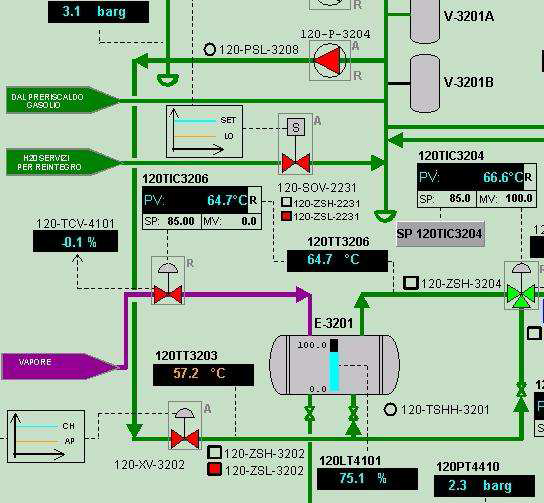
Figure 2. Overview of part of the renewable energy plant used for experimental results.

Figure 3. Set-point step responses in the temperature control loop. Left: initial; right: retuned.

Conclusions

Methodologies for the deterministic performance assessment and retuning of PID controllers have been reviewed and presented in a unified way in this paper. The basic idea, developed for different contexts, is to exploit the final value theorem to estimate the process parameters based on the integral of appropriate signals that results from a set-point or a load disturbance step response. This makes the technique suitable for implementing in industry, as it uses routine operating data, and is inherently robust to measurement noise and the result is almost independent of the tuning of the initial controller (on the contrary, standard least squares techniques assume an input signal that significantly excites the dynamics of the system to be estimated). The methodologies analyzed can be implemented with standard Distributed Control Systems software and can also be extended to more complex control techniques, like cascade control, dead time compensators and feedforward control.

Despite the enhanced multivariable control available algorithms, which computation complexity typically needs to be implemented at upper level, PID control is still the primary component of any basic loop and through clever PID-based architectures many “DCS-enabled” solutions can be built up and standardized in the industry. Therefore PID control will still be used for long time; its knowledge will still be a key for any control/process engineer, and any contribution for improving the effectiveness of PID control will always be welcome both in research and in the industry.

Learn more about Yokogawa's Regulatory Control Stabilization solution and TuneVP software

An overview of this methodology can be found on-line:

M. Veronesi, A. Visioli, Deterministic Performance Assessment and Retuning of Industrial Controllers Based on Routine Operating Data: Applications – www.mdpi.com/journal/processes